Using Regression to Blur an Image
Perhaps the most challenging to implement, this section originally started out as an attempt to colorize grey scale images by predicting color values based on a similiar image's pixel locations. Two different approaches were utlized here, one with multivariate linear regression, and one with multivariate polynomial regression. Linear regression was more straight foward in implementation but had rather unfavorable results. Polynomial regeression on the other hand gave some interesting results, but required testing several different degrees for the polynomials used. The difficulties encountered in trying to colorize images using this approach was overlaying the predicted colors onto the original grey scale image. This will be discussed in more detail in the Process section, but hitting this barrier resulted in modifying the code and recognizing that it produced blurred, colorized, images with very little traits of the original image. Little visible traits of course is favorable in concealing an identity when blurring an image, therefore implying the code did its job! Something to note as well was that images of poor resolution did not fair well in passing through the algorithm as well. (ADD OVERLEAF THEORY PIC on polynomial regression)
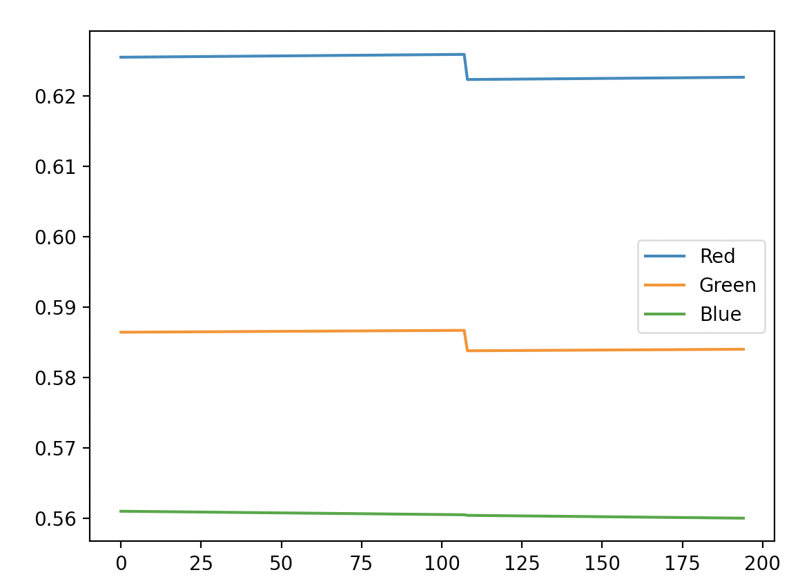
Process for Linear Regression
- 1. Read in colored PNG image with Matplotlib and convert it to a numpy array. We then scale the image down by a factor of 4 to speed up the process.
- 2. Find the dimensions of our image where m is the number of rows and n is the number of columns
- 3. Create a Pandas data frame with the following 5 columns: X coordinate, Y coordinate, red value, green value, blue value
- 4. Check that the dimensions of the data frame is m*n rows by 5 columns
- 5. Perform multivariate linear regression with the X coordinate and Y coordinate columns serving as the explantory variables and the color values being the response variables
- - note: since we have 3 color channels, the followibg procedure is performed 3 times.
- 6. This entails using sklearn's LinearRegression function to obtain a y-intercept, coefficents at each (x,y) coordinate, and create a trend line
- 7. Next the predicted red, green, and blue values are predicted by plugging in each (x,y) coordinate from the original image
- - note: we obtain 3 seperate arrays for predicted red, green, and blue values as there is a trend line for each color channel
- 8. Use python's zip function on the three arrays to create an array of touples where each touple represents a pixel's rgb values
- - note: the structure of this array is [(r,g,b)...(r,g,b)]
- 9. Append 1 to each touple in order to include the intensity channel at each pixel.
- 10. Shape the array of predicted touples into the same dimensions as our original image
- 11. For each pixel in the original image, overwrite it with the aquired predicted pixel as given by the linear regression procedure
- 12. The process is now complete but as noted in the description, it isnt very flattering!
Example


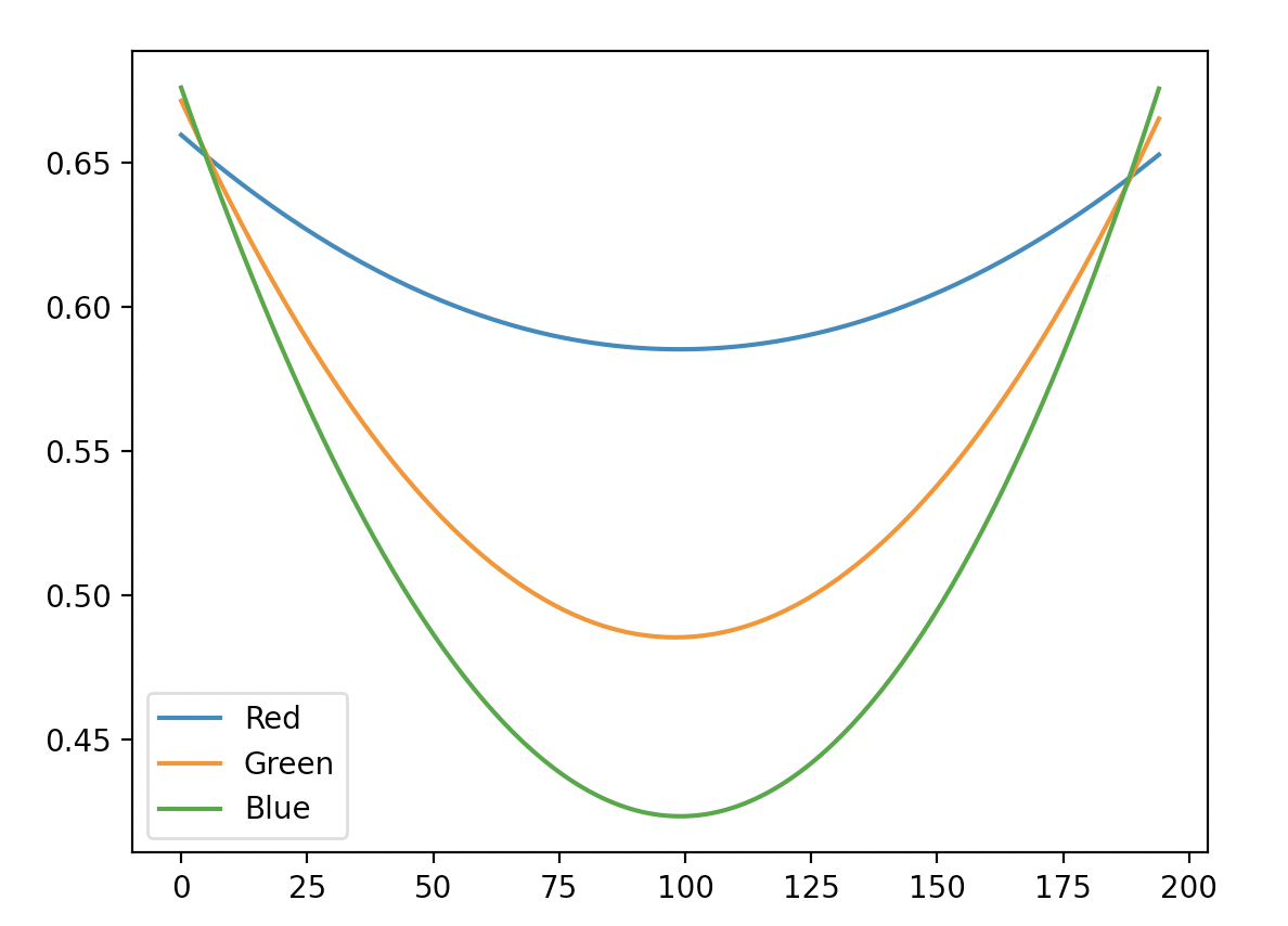
Process for Polynomial Regression
- 1. Steps 1-4 are the same as the procedures explained in the linear regression example.
- 5. Perform multivariate polynimial regression with the X coordinate and Y coordinate columns serving as the explantory variables and the color values being the response variables
- - note: since we have 3 color channels, the following procedure is performed 3 times.
- 6. Use sklearn's PolynomialFeatures and LinearRegression functions to transform our explantory variables, fit our new data, and then predict our color values.
- 7. Pick the largest possible degree of polynomial as that will reveal the "most" features in our blurred image. The lower the degree polynomial, the less features become visible.
This is neccessary as each degree produces different coefficients for our lines of fit and as a result certain predicted color values fall outside of the range [0,1].
This implies python will not be able to read invalid color values into our resulting image.
- - note: Step 7 was done as a trial and error method, however this can be implemented by cycling through polynomials of incrimented degrees and
checking if any of the resulting predicted pixels contain either negative values or values greater than 1.
- 11. Steps 7-11 are the same as the procedures explained in the linear regression example.
- 12. The process is now complete and as noted in the description, is much more flattering than that of linear regeression!
Example